Optical Anti-Icing: CNN Ice Detection on Turbine Inlets

Executive summary

This is the ice-detection work on my resume. In cold, moist weather, ice can form on the inlet guide vanes at the front of a gas turbine. If that ice builds to a critical mass and then sheds into the compressor, it can do hundreds of thousands or millions of dollars of damage. Plants already protect against that with inlet bleed heat (IBH): when weather conditions indicate an icing risk based on empirical evidence, a control schedule triggers the IBH. It siphons warm air from later compressor stages and puts a temperature offset on the inlet to get it above freezing. That heat is not free — it comes out of the compressor which did work to heat the air, and a hotter inlet is a less efficient machine — so GE wanted to know whether a camera and a convolutional neural network (CNN) on the edge could see ice on the vanes and run IBH with that in closed-loop control, as opposed to the existing, conservative, open-loop schedule.

In winter of 2023, GE’s Advanced Research Center (ARC) in Niskayuna, NY, showed that a model could be trained on inlet icing images, which is the first thing you have to believe before you put a camera in a control loop. In summer 2025 that proof of concept landed at my desk on the advanced controls team with the trained weights gone and the code scattered to the wind. I was told to find the code and the data, train new models, write the documentation, figure out how the estimated ice coverage would talk to the controller, and put a business case together. I owned the whole thing.

Those models had to turn a camera frame of the inlet into ice coverage a controller could read. I trained two convolutional networks (U-Nets) on the annotated images: one to mark the vanes, so ice on the inlet wall would not count, and one to mark ice. OpenCV then split the vane mask into individual vanes and intersected it with the ice, which is how you get total and per-vane percent coverage. I rebuilt ARC’s training code so that work could be repeated after the original weights were lost, expanded on their blur check so a bad frame would fall back to the weather schedule, and timed the exported inference loop on a small, resource-capped box. Median overlap with the labeled masks (IoU), on a random test split from that camera, was 1.00 for vane area, 0.75 for edges, and 0.71 for ice. Those numbers are hard to conceptualize without their accompanying images, but informally I’d say the models were “pretty darn good.”

The camera’s only dollar job is to spend less IBH than the schedule already spends. Based on a real icing site’s winter 2024–2025 hours, I calculated that eliminating all scheduled bleed heat (which would be the theoretical best case scenario) is worth ~$77k per unit per year on a 7F and ~$170k on a 7HA. A camera could only claim an estimated 5–20% of that, since the default schedule was already near icing the icing threshold. Based on those calculations, I unofficially recommended we not proceed, while I deferred to the program manager. Ultimately, the program was killed.

The product problem: ice on inlet guide vanes, and IBH that is not free

Those vanes sit at the compressor face: the left side of a machine like the one below.

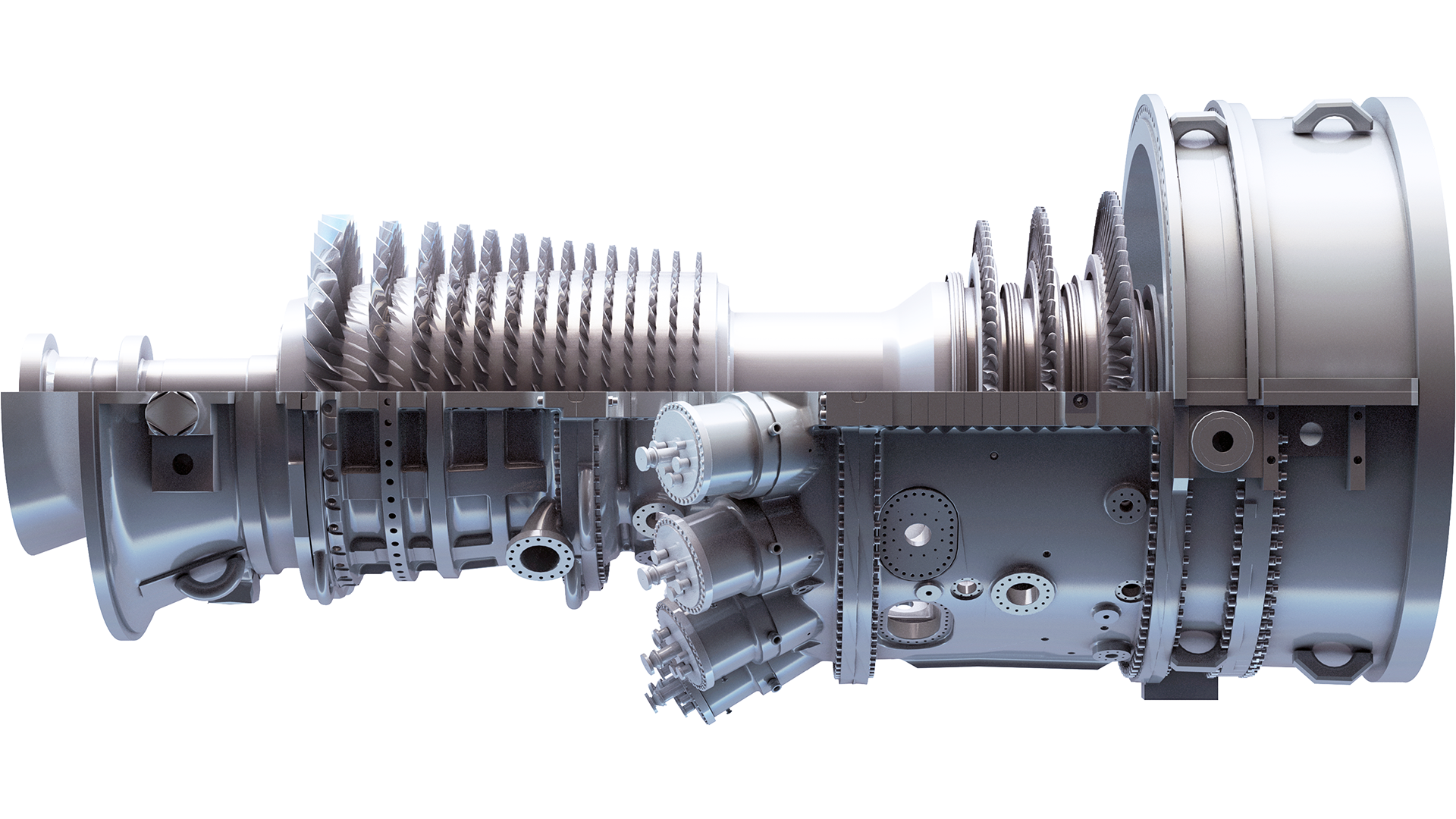
If ice sheds off those vanes, it goes into that compressor, whose blades are thin, spinning, and intolerant of a slab of ice. A damaged compressor looks like this:

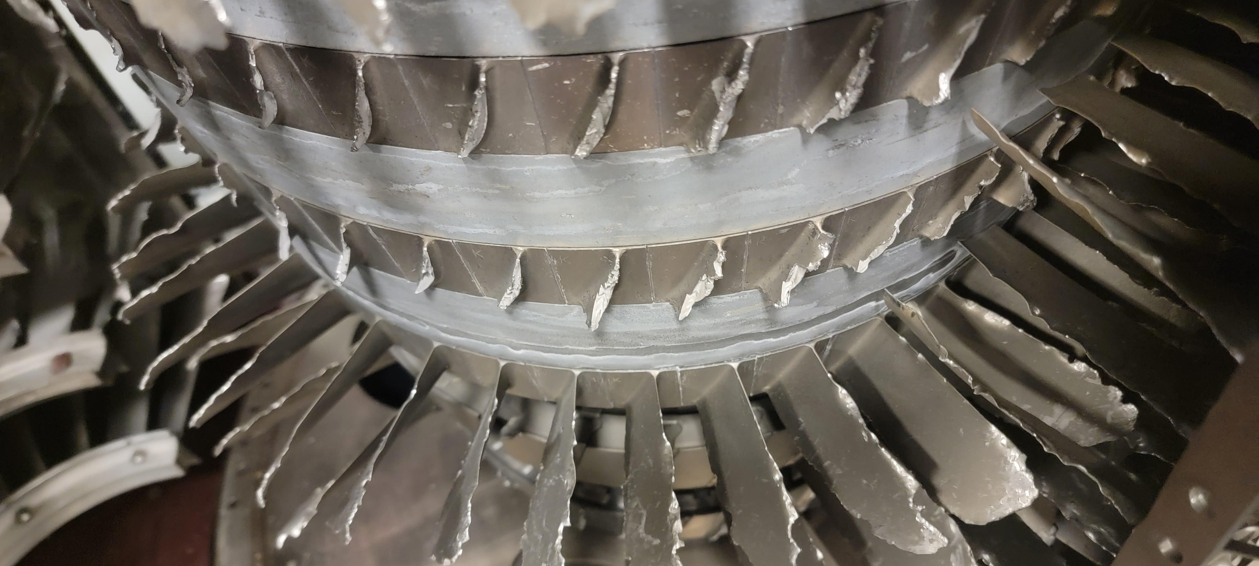
The plant’s current protection is that weather-driven control schedule. IBH is still the only tool, but as mentioned, the heat is leeched from the turbine and a hotter inlet reduces efficiency. Thus, less IBH is better as long as you do not corn-cob a compressor.

ARC’s first cut was whether a model could even see the ice. Their proof of concept used a small dataset — about 2,000 annotated images, covering around 10 separate icing events, from one pilot site — and in winter 2023 that was enough to show a model could be trained. The weights themselves did not survive, so what advanced controls inherited a year and a half later was an example training pipeline and the annotated images.

I had to understand that pile well enough to change it, not just rerun it: train new weights, quantify accuracy and failure modes, and split the work into offline training infrastructure and an inference pipeline.

Handoff: a proof of concept, no weights, spaghetti

The first month was archaeology rather than training. The ARC had already gathered the images, annotated them, and left an example pipeline that proved the science was not crazy. I just had to find it and piece together the story from a project that had collected dust for two years. The ARC proof of concept was a great starting point, even though it was also a copy-pasted, hardcoded spaghetti mess — frankensteined from a pile of other projects, meant to get something out the door, not to be robust, organized, or comprehensible. I did not invent the two-model ice/vane idea; I read it, modified it, and took it far enough that it could be trained, evaluated, and argued about as a product. The trained weights themselves were lost, and there was no clean handoff package sitting in a repo with a README.

Inference pipeline

The inference pipeline starts with an image of the inlet of the turbine. That image goes through two models, then OpenCV post-processing, then a handful of scalar metrics the controller can use.

%%{init: {"flowchart": {"htmlLabels": true, "wrappingWidth": 160, "useMaxWidth": true}}}%%
flowchart TD
    Cam(Inlet camera frame)
    Gate{Blur / image-quality gate}
    Fallback(Wait for next image)
    Sharp(sharp)
    Vane("<strong>Dual-layer U-Net</strong><br><em>EfficientNetB4</em><br>vane area and edges")
    Ice("<strong>Ice U-Net</strong><br><em>EfficientNetB4</em><br>ice pixels")
    OpenCV("<strong>OpenCV:</strong> split area mask<br>into vanes using the edge mask")
    Intersect("Ice mask intersect<br>per-vane regions")
    Metrics("Total percent ice and<br>max individual-vane percent ice")
    Ctrl("<strong>Controller:</strong> value and rate<br>of change drive IBH")

    Cam --> Gate
    Gate -->|blurry| Fallback
    Gate -->|sharp| Sharp
    Sharp --> Vane
    Sharp --> Ice
    Vane --> OpenCV
    OpenCV --> Intersect
    Ice --> Intersect
    Intersect --> Metrics
    Metrics --> Ctrl

Why two models, not one “ice on vanes” net. The camera also sees the inlet walls, so vane-area and vane-edge masks let you restrict ice to the vanes the which the compressor actually cares about, and they let you report per-vane coverage instead of a single blob.

Why OpenCV after the nets. Segmentation gives pixels, and the control system cannot eat a mask. Splitting the area mask along the edge mask produces individual vanes; intersecting those regions with the ice mask produces per-vane ice. From there you get:

• total % ice coverage across the visible vanes (the camera sees ~1/6 of the inlet)
• max individual-vane % ice coverage (one vane icing hard while the average still looks fine)

Those scalars are what would be published into the control system. The controller looks at coverage over time — both the value and the rate of change — and decides whether IBH needs to come on to stop an icing event. If the optical path dies, IBH reverts to the slightly conservative weather schedule so a camera or model failure cannot become a compressor event.

That is the product loop: a camera estimate that can turn IBH on, and a schedule that takes over if the optical path dies.

The four technical questions

The business case asked whether this was worth attaching to a turbine. These four asked whether the measurement was even a measurement, which is why a model that works on the pilot images can still be unshippable. Keep in mind that one site, ~10 icing events, and ~2,000 frames make up the entire evidence base for all four answers.

Site-to-site variation

The proof of concept saw one inlet, one camera mount, one climate, and one lighting setup. A fleet product has to survive the next site; if it does not, you are selling a per-plant science project rather than a control feature.

What actually changes when you leave the pilot is inlet/blade condition (rust, wear), camera and aim, lighting and glare, rime vs glaze ice, and background clutter.

We had no data from a second site, not even unlabeled frames, so I wanted at least three sites — more data, new models — before a second call on fleet-readiness. One generalized model was the ideal, but the evidence we had was one camera on one inlet, which means the model learned this camera on this inlet, not “ice.”

Model robustness

Accuracy is performance on the labeled distribution, whereas robustness is what happens when the camera leaves that distribution. One problem that we encountered and overcame was blurriness in the source images.

Blur Detection Study

The pipeline had an image-quality gate before the ice/vane nets, because people at the ARC had already ran into a blurriness problem and manually tagged blurry vs sharp frames to train a blur detection model. I compared five blue detectors on that image set, then put the winner in front of the inference pipeline as shown above in the flow chart to help the overall inference pipeline be more robust to noise.

Blur Detection Method	What it uses	Knobs
Laplacian variance	Sharp = high variance	threshold
FFT high-frequency energy	Sharp = more high-frequency power	cutoff between high/low, energy-ratio threshold
Tenengrad / Sobel	Sharp = high edge (gradient) magnitude	magnitude threshold
skimage.measure.blur_effect	skimage’s blur score	h_size
Custom CNN	EfficientNetB1 + pooling + dropout	trained with categorical CE

The classical blur detection methods are mostly scalar calculations that aggregate some information about the image, and usually depend on some tuning parameter. For instance, if you calculate the Laplacian variance for an image, you get out a single number, and you then have to decide if that number represents a blurry or sharp image by setting some threshold. I needed a way to tune the hyperparameters for these models, so I turned towards a ubiquitous machine learning libary, scikit-learn.

scikit-learn (sklearn) is a Python library built for training and comparing machine learning models, but its tools — grid search, cross-validation, threshold tuning — only work on objects that look like sklearn’s classifiers. I wrapped each blur detector as one of those sklearn objects: a class that inherits sklearn’s BaseEstimator and ClassifierMixin, which is the pair that tells sklearn this thing can be fit and can predict a class.

You cannot tune a method’s knobs and then report accuracy on the same split, so they were tuned with nested stratified k-fold cross-validation. The inner loop grid-searches the method-specific hyperparameters — Laplacian’s threshold, FFT’s cutoffs, the CNN’s training knobs — on training folds, and the outer loop holds data out to prevent overfitting. Stratified means each fold keeps the ratio of the global blurry/sharp mix.

Running the sklearn training pipeline on the traditional blur detection methods gave me 4 of the traditional blur-detection methods plus the one 1 neural network I had from my neural network pipeline, all trained on the blurry/sharp image set. Each of those models took in an image of the inlet and output a number between 0 and 1 which represented the sharpness of the image. I then added sklearn’s TunedThresholdClassifierCV, which picks where the cutoff between 0 and 1 should be for blurry and sharp. I plotted precision-recall (PR) curves and model-complexity curves, and ultimately the CNN won the battle as the best blur detection method.

Ultimately, model robustness was a large unknown in the project and I raised those concerns early and often. I highlighted the risk that a single-site dataset posed with regards to our understanding of if the model would be universal. I did, however, attempt to mitigate that risk by adding image augmentation to our model training pipeline, as described later in the article.

Model accuracy

To score the three networks I used intersection over union (IoU), which is a standard segmentation metric. You overlay the model’s predicted mask on the human-labeled mask, and IoU is the area they share divided by the area of their union, so 1.00 is a perfect overlay and 0 is no overlap at all. When you train a model you usually split the labeled images into three piles: a training set the optimizer sees, a validation set you watch while you are still picking hyperparameters, and a test set you hold back until the end so the number you quote is not the one you optimized against. The medians in the table below are from that test split. The split itself was random frames drawn from the same ~2,000-image pile — some iced, some clear — which means a frame from a given icing event could sit in training while its neighbor from a few seconds later sat in test. Holding out an entire icing event, or frames from a second site, would have been a stricter check, and we did not have the data to do that.

Model	Median IoU (test)
Vane area	1.00
Vane edges	0.75
Ice segmentation	0.71

On that table the ice model looks worse than the vane models. Looking at the frames next to the masks, though, the ice overlays were good enough: the model was finding the ice you can see in the photo, even when the overlap score sat below area and edges.

Frames from one icing event are correlated in time and lighting, so a random image split can put neighbors in train and test and make the test number look more optimistic than a true held-out event would. These IoUs say the model works on this camera, at this site, on frames that look like the rest of the pile, including clear days. They leave open whether it works on the next icing event, the next site, or the five-sixths of the inlet the camera cannot see, which is why site-to-site variation and coverage still sat next to the accuracy numbers when we were deciding whether to ship.

IoU also does not tell you whether percent ice is high or low, because a mask can overlap the label reasonably well and still be systematically a little large or a little small. The controller uses that percent, so I needed a check on the scalar itself. I ran the same quantification analytic on model masks and on ground-truth masks and put the pairs on a parity plot in Plotly, so that if the model were honest the points would sit on the diagonal.

The plot showed a consistent ~5% overprediction: coverage derived from the model masks sat above coverage derived from the ground-truth masks. If you treated the labels as truth, that bias would have gone straight into the IBH decision.

I made the plot clickable so that clicking a point brings up three images — the base frame, the ground-truth mask, and the model mask — which is how you decide whether the model is wrong or the label is incomplete. Outliers I could reject by eye. The systematic 5% was coming from underlabeled ground-truth masks: the labels stopped short of the ice you can see in the photo, and the model was closer to the photo. That is also why the ice IoU looked worse than the pictures felt, because some of the overlap miss is the label being small.

Model coverage

Even if the masks are good on the frames we have, the camera still only sees about one-sixth of the inlet. That field of view is a product choice as much as a camera spec, because you then have to decide whether to install six cameras — extra ports, enclosures, lighting, install, and more streams — or to assume icing is uniform around the inlet and treat the visible sixth as a sample of the whole.

If icing really is even around the circumference, one camera is enough to speak for the compressor. Windward versus leeward sides, sun, local geometry, or a blocked sector can break that, and then the model can be perfect on the vanes it sees and still miss the ice that sheds. Pixel metrics on the visible sixth will never show that miss.

The CNN cannot answer that from the pilot field of view, because the ~10 events were all filmed from the same sixth. It is an instrumentation and physics question: a second camera angle, operator evidence, or computational fluid dynamics (CFD) that icing is even around the inlet.

It is also a compute question, which I get to in the timing section below. 1.6 frames per second on eight CPU cores is enough for one camera, given that humidity icing happens on a scale of minutes. Six cameras at that same throughput would not be, because you would be splitting the budget across six streams. Rejecting uniformity therefore multiplies both the install bill of materials and the edge compute, which is the point at which a GPU enters the conversation.

Uniformity was an open assumption. We did not have a second camera angle, operator proof, or CFD that icing is even around the inlet. One camera is only a sensor if you grant that assumption. If you do not, you are buying six cameras and the compute to run them, and the ~$77k ceiling on a 7F does not pay for that. We never closed whether the visible sixth is allowed to speak for the compressor, so we never closed whether one camera is enough.

Business case

The four questions above asked whether the measurement was honest. Separate from that, the weather schedule already spends IBH to keep ice off the vanes, so this product does not add a new kind of protection. The camera’s only dollar job is to spend less IBH than that schedule already spends. The physics-bound ceiling is therefore what all of today’s scheduled IBH costs the customer for a winter, on a real site. Anything the model can claim is a fraction of that ceiling, and if the ceiling is only tens of thousands of dollars a year, there is not much room left for a camera product.

The method was to pick a real customer site that ices, then pull winter 2024–2025 operating hours into four ambient temperature buckets that actually had runtime. For each bucket, I ran the included plant simulation twice: once with the default IBH schedule on, and once with IBH off. That gives heat rate and output at those ambients, with and without bleed heat.

From heat rate, output, and hours actually run at those temperatures and loads, I computed power generated and operating expenditure. At baseload, generated power times $0.05/kWh ($50/MWh) minus operating expenditure is profit with IBH versus without. That $/kWh was an assumed market levelized cost of energy (LCOE). I pulled the figure from Google on 20 November 2025, because I did not have that site’s power purchase agreement or its locational marginal price. At a representative part-load, I compared operating expenditure with versus without IBH. The profit gap at baseload plus the operating-expenditure gap at part-load is the cost of IBH to that customer.

Because the optical loop can only reduce IBH, and cannot beat a plant that never turns it on, that IBH cost is the theoretical ceiling on value per unit per year.

Class	Theoretical ceiling (all IBH eliminated)
7F	$77k / unit / year
7HA	$170k / unit / year

The camera would never capture the whole ceiling, because it cannot turn IBH off in conditions where the schedule was right to have it on. The 5–20% slice I quoted was a gut band: I did not count hours where IBH was on and there was no ice. The schedule was probably already close to the icing line, because if they lower it much more, they get icing. Most of the IBH it spends is therefore doing real work, so the camera is arguing about a thin remaining margin. On a 7F that sketch is about $4–15k per year. I presented the ceiling and the band as they were.

When the review asked what I recommended, I said unofficially, do not proceed, on lack of customer added value, and officially I deferred to the program manager, who killed the program.

This case prices IBH fuel and output, because the schedule already exists to prevent sheds. Adding a million-dollar ingest that the schedule is already paid to stop would be double-counting protection this camera does not add.

Model architecture and training

The nets in the inference pipeline were U-Nets with an EfficientNetB4 backbone, in Keras / TensorFlow. B4 was the ARC default from the proof of concept, so I kept it and did not sweep other backbones. The vane net is one U-Net with a multi-layer output: each output channel is one mask (area, edges). A pixel can be area and edge, which is multi-label: the same pixel can belong to more than one class, so you do not need two separate nets, and you do not use a softmax that would force the pixel into a single class. Ice is a second U-Net-B4, binary.

My custom SegmentationTrainer class could run binary cross-entropy (BCE), Dice, BCE+Dice, categorical cross-entropy (CCE), and CCE+Dice, so I could compare them and pick a loss that matched binary versus multi-label. I settled on BCE+Dice for both ice (binary) and vane (multi-label). BCE pays per pixel; Dice pays for overlap, which matters when ice is a tiny fraction of the image.

EfficientNet is a family of image-classification backbones that scale depth, width, and input resolution together, from B0 (smallest) through B7 (largest). B4 is a mid-heavy ImageNet encoder: more floating-point operations and parameters than B0 or B1, and usually better features. Segmentation runs that encoder plus a decoder that upsamples back to a mask, so CPU time is mostly the backbone. The blur detector, which is a whole-image call rather than a pixel mask, used B1 and no decoder, which is a cheaper job. We did not try B0 or B1 for ice and vane. Eight-core CPU at 1.6 FPS was already enough for one camera, so a smaller encoder would have been optional headroom, and would have mattered more for six streams. I did not measure that delta.

After the proof-of-concept weights were lost, the work was making this stack trainable, comparable, and exportable again. ARC’s example was spaghetti, and this is the stack that could actually train more than once.

An analysis pipeline looped the same functions over different configuration sets so I could train multiple models and compare them without forking the script. A SegmentationTrainer took a SegmentationModelConfig — a Pydantic BaseModel. Pydantic is a Python library for typed data models that validate on construction, so the knobs were typed, documented, and fail-closed if you omitted one. The repo was type-checked and linted. Pydantic modeled the data, not just the trainer config.

The train method used a custom segmentation data generator that subclassed Keras Sequence, which is Keras’s interface for feeding batches during fit. Each step loaded a batch of images plus masks and fed the fit loop. On that path I used Albumentations, an image-augmentation library, for:

• horizontal flip
• one of affine or perspective
• one of Gaussian or median blur
• random brightness / contrast
• HueSaturationValue

The augmentations were geometric and photometric jitter, plus blur. I did not mix images together to synthesize fake ice. The blur augmentation during training and the blur gate at inference are complementary: the net can survive mild smear, while the gate still refuses a garbage frame.

The config loop was mostly a loss sweep over the five losses above, which is how I compared models with the same code. I kept BCE+Dice.

Training ran on an existing RTX 4090 for about 10 hours, aimed at one generalized model.

Compute

Those 10 hours on the RTX 4090 are for offline training, so speed doesn’t matter much. The plant would run inference, and that is the product constraint, because the edge box is not a 4090, and we did not get to pick a hefty GPU without a cost argument.

I timed the full pipeline, including the ONNX models plus the ice quantification analytic that turns masks into percent ice, which is the same loop the controller would see. ONNX is an export format so you can run a Keras model without shipping TensorFlow to the edge.

To make the numbers look like a small edge box, I put the pipeline in Docker and artificially constrained the container’s CPU count and RAM. The design of experiments covered 1–16 CPUs and 512–2048 MB RAM. Average frames per second (FPS) was the metric. I plotted that as a 3D surface (FPS versus cores versus memory). Then I repeated the same pipeline against a low-end laptop GPU (Quadro T1200) and against the 4090, still sweeping cores and memory. On the GPU the cores axis was almost flat: extra CPUs helped only marginally, because the nets were no longer the CPU’s job.

Loading interactive FPS plot…

On CPU-only runs, memory moved the needle a little: more RAM was slightly faster, without changing the cores shape.

CPUs	Approx. FPS	Period
1	~0.25	~4 s/frame
8	~1.6	~0.6 s/frame
16	~2	~0.5 s/frame

Returns diminished after 8 cores. Constraining RAM made it slightly slower without changing the shape.

With a GPU, memory only mattered when severely constrained:

Device	RAM	Approx. FPS
Quadro T1200 (low-end laptop)	constrained	~5.2
Quadro T1200	≥ 1 GB	~6
RTX 4090	—	~9

The T1200 is about 2/3 the FPS of the 4090 at about 1/3 to 1/4 the cost. If we decided the product needed a GPU, I recommended the cheap one. A 4090 in the turbine cabinet would be training-class silicon for an inference job that the T1200 already covers.

How fast is fast enough depends on how quickly ice can grow, which is a physics question.

Humidity-based icing happens on the order of minutes. For a single camera, 1.6 FPS on 8 CPU cores is enough, because you are sampling hundreds of times per icing time constant. Precipitation-based icing, for example freezing rain, can be much faster, and would need a shorter iteration time.

Six cameras change the throughput you need, because 1.6 FPS is a one-stream number, and split across six views it is not enough. Coverage and compute are therefore the same decision: if you assume uniformity, a CPU box is in the hunt; if you reject uniformity, you are buying cameras and a GPU, still the cheap one rather than a 4090.

Control-system integration

None of that ran closed-loop on a turbine. The intent was to publish total percent ice and max-vane percent ice, plus refuse-on-blur, so that value and rate of change would drive IBH, while a dead optical path falls back to the schedule.

The tag bus was not built out. Icebox, the OPC-UA to MQTT adapter in the card below, would have been one way those scalars left the box. Icebox moves tags from one protocol to another; this work estimates ice. They would have sat next to each other, but they are different products despite the coincidence of “ice” in the name “Icebox.”